Logistic distribution is ones of the most widely used distributions in statistics. Even though we are not conscious of it, we are using the logistic distribution whenever we do logistic regression. The frequentist way of fitting a logistic model is quite straightforward. However, the Bayesian logistic model isn’t quite as easy due to its non-conjugacy. In those cases, it is very useful to use the hierarchical representation of the distribution. This post is aimed at reviewing 2 types of modelling logistic regression in a Bayesian way.
The first is to use the logistic distribution directly. Choi and Hobert (2013) proposes a Gibbs sampler using the Polyá-Gamma distribution which isn’t easy to sample from. Those who are interested in the random variate generation algorithms are referred to Devroye (1986). In fact, Devroye released the book free of charge online (here). Anyway, let’s review logistic regression briefly. The probability density function (PDF) of a logistic distribution is as follows:
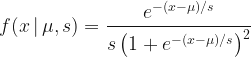
for location parameter 


Such a function 

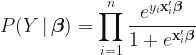
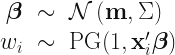
For simplicity, let’s assign a standard multivariate normal distribution for 
![\pi(\boldsymbol{\beta}\,|\,Y) \propto \left[\displaystyle\prod_{i=1}^{n}\dfrac{e^{y_{i}\mathbf{x}_{i}'\boldsymbol{\beta}}}{1+e^{\mathbf{x}_{i}'\boldsymbol{\beta}}}\right]e^{-\boldsymbol{\beta}'\boldsymbol{\beta}/2}](https://s0.wp.com/latex.php?latex=%5Cpi%28%5Cboldsymbol%7B%5Cbeta%7D%5C%2C%7C%5C%2CY%29+%C2%A0%5Cpropto+%5Cleft%5B%5Cdisplaystyle%5Cprod_%7Bi%3D1%7D%5E%7Bn%7D%5Cdfrac%7Be%5E%7By_%7Bi%7D%5Cmathbf%7Bx%7D_%7Bi%7D%27%5Cboldsymbol%7B%5Cbeta%7D%7D%7D%7B1%2Be%5E%7B%5Cmathbf%7Bx%7D_%7Bi%7D%27%5Cboldsymbol%7B%5Cbeta%7D%7D%7D%5Cright%5De%5E%7B-%5Cboldsymbol%7B%5Cbeta%7D%27%5Cboldsymbol%7B%5Cbeta%7D%2F2%7D+&bg=%23ffffff&fg=%23111111&s=1&c=20201002)
The trick here is to introduce another random variable that is totally irrelevant if 


![\begin{array}{lcl} \pi(\boldsymbol{\beta}\,|\,Y) &\propto & \left[\displaystyle\prod_{i=1}^{n}\dfrac{e^{y_{i}\mathbf{x}_{i}'\boldsymbol{\beta}}}{1+e^{\mathbf{x}_{i}'\boldsymbol{\beta}}}\right]e^{-\boldsymbol{\beta}'\boldsymbol{\beta}/2}\\ \pi(\boldsymbol{\beta},w\,|\,Y) &\propto&\left[\displaystyle\prod_{i=1}^{n}\dfrac{e^{y_{i}\mathbf{x}_{i}'\boldsymbol{\beta}}}{1+e^{\mathbf{x}_{i}'\boldsymbol{\beta}}}\times \dfrac{1+e^{\mathbf{x}_{i}'\boldsymbol{\beta}}}{2e^{\mathbf{x}_{i}'\boldsymbol{\beta}}}e^{-\frac{(\mathbf{x}_{i}'\boldsymbol{\beta})^{2}w_{i}}{2}}g(w_{i}) \right]e^{-\boldsymbol{\beta}'\boldsymbol{\beta}/2}\\ g(w) &=& \displaystyle\sum_{k=0}^{\infty}(-1)^{k}\dfrac{(2k+1)}{\sqrt{2\pi w^{3}}}e^{-\frac{(2k+1)^{2}}{8w}}\mathbb{I}_{(0,\infty)}(w) \end{array}](https://s0.wp.com/latex.php?latex=%5Cbegin%7Barray%7D%7Blcl%7D+%5Cpi%28%5Cboldsymbol%7B%5Cbeta%7D%5C%2C%7C%5C%2CY%29+%26%5Cpropto+%26+%5Cleft%5B%5Cdisplaystyle%5Cprod_%7Bi%3D1%7D%5E%7Bn%7D%5Cdfrac%7Be%5E%7By_%7Bi%7D%5Cmathbf%7Bx%7D_%7Bi%7D%27%5Cboldsymbol%7B%5Cbeta%7D%7D%7D%7B1%2Be%5E%7B%5Cmathbf%7Bx%7D_%7Bi%7D%27%5Cboldsymbol%7B%5Cbeta%7D%7D%7D%5Cright%5De%5E%7B-%5Cboldsymbol%7B%5Cbeta%7D%27%5Cboldsymbol%7B%5Cbeta%7D%2F2%7D%5C%5C+%5Cpi%28%5Cboldsymbol%7B%5Cbeta%7D%2Cw%5C%2C%7C%5C%2CY%29+%26%5Cpropto%26%5Cleft%5B%5Cdisplaystyle%5Cprod_%7Bi%3D1%7D%5E%7Bn%7D%5Cdfrac%7Be%5E%7By_%7Bi%7D%5Cmathbf%7Bx%7D_%7Bi%7D%27%5Cboldsymbol%7B%5Cbeta%7D%7D%7D%7B1%2Be%5E%7B%5Cmathbf%7Bx%7D_%7Bi%7D%27%5Cboldsymbol%7B%5Cbeta%7D%7D%7D%5Ctimes+%5Cdfrac%7B1%2Be%5E%7B%5Cmathbf%7Bx%7D_%7Bi%7D%27%5Cboldsymbol%7B%5Cbeta%7D%7D%7D%7B2e%5E%7B%5Cmathbf%7Bx%7D_%7Bi%7D%27%5Cboldsymbol%7B%5Cbeta%7D%7D%7De%5E%7B-%5Cfrac%7B%28%5Cmathbf%7Bx%7D_%7Bi%7D%27%5Cboldsymbol%7B%5Cbeta%7D%29%5E%7B2%7Dw_%7Bi%7D%7D%7B2%7D%7Dg%28w_%7Bi%7D%29+%5Cright%5De%5E%7B-%5Cboldsymbol%7B%5Cbeta%7D%27%5Cboldsymbol%7B%5Cbeta%7D%2F2%7D%5C%5C+g%28w%29+%26%3D%26+%5Cdisplaystyle%5Csum_%7Bk%3D0%7D%5E%7B%5Cinfty%7D%28-1%29%5E%7Bk%7D%5Cdfrac%7B%282k%2B1%29%7D%7B%5Csqrt%7B2%5Cpi+w%5E%7B3%7D%7D%7De%5E%7B-%5Cfrac%7B%282k%2B1%29%5E%7B2%7D%7D%7B8w%7D%7D%5Cmathbb%7BI%7D_%7B%280%2C%5Cinfty%29%7D%28w%29+%5Cend%7Barray%7D+&bg=%23ffffff&fg=%23111111&s=1&c=20201002)
Let’s not care about that ugly function 
the joint posterior 
![\pi(\boldsymbol{\beta},w\,|\,Y) \propto \left[\displaystyle\prod_{i=1}^{n}\dfrac{e^{y_{i}\mathbf{x}_{i}'\boldsymbol{\beta}}}{1+e^{\mathbf{x}_{i}'\boldsymbol{\beta}}}\times \cosh\left(\dfrac{|\mathbf{x}_{i}'\boldsymbol{\beta}|}{2} \right)e^{-\frac{(\mathbf{x}_{i}'\boldsymbol{\beta})^{2}w_{i}}{2}}g(w_{i}) \right]e^{-\boldsymbol{\beta}'\boldsymbol{\beta}/2}](https://s0.wp.com/latex.php?latex=%5Cpi%28%5Cboldsymbol%7B%5Cbeta%7D%2Cw%5C%2C%7C%5C%2CY%29+%5Cpropto+%5Cleft%5B%5Cdisplaystyle%5Cprod_%7Bi%3D1%7D%5E%7Bn%7D%5Cdfrac%7Be%5E%7By_%7Bi%7D%5Cmathbf%7Bx%7D_%7Bi%7D%27%5Cboldsymbol%7B%5Cbeta%7D%7D%7D%7B1%2Be%5E%7B%5Cmathbf%7Bx%7D_%7Bi%7D%27%5Cboldsymbol%7B%5Cbeta%7D%7D%7D%5Ctimes+%5Ccosh%5Cleft%28%5Cdfrac%7B%7C%5Cmathbf%7Bx%7D_%7Bi%7D%27%5Cboldsymbol%7B%5Cbeta%7D%7C%7D%7B2%7D+%5Cright%29e%5E%7B-%5Cfrac%7B%28%5Cmathbf%7Bx%7D_%7Bi%7D%27%5Cboldsymbol%7B%5Cbeta%7D%29%5E%7B2%7Dw_%7Bi%7D%7D%7B2%7D%7Dg%28w_%7Bi%7D%29+%5Cright%5De%5E%7B-%5Cboldsymbol%7B%5Cbeta%7D%27%5Cboldsymbol%7B%5Cbeta%7D%2F2%7D+&bg=%23ffffff&fg=%23111111&s=1&c=20201002)
Surprisingly, 


![\begin{array}{lcl} \pi(\boldsymbol{\beta}\,|\,w,Y) &\propto& \left[\displaystyle\prod_{i=1}^{n} \exp\left(y_{i}\mathbf{x}'\boldsymbol{\beta}-\dfrac{\mathbf{x}_{i}'\boldsymbol{\beta}}{2}-\dfrac{w_{i}\boldsymbol{\beta}'\mathbf{x}_{i}\mathbf{x}_{i}'\boldsymbol{\beta} }{2}\right)\right]e^{-\boldsymbol{\beta}'\boldsymbol{\beta}/2}\\ &=& \exp\left(Y'X\boldsymbol{\beta}-\dfrac{\boldsymbol{\beta}'X\mathbf{1}}{2}-\dfrac{\boldsymbol{\beta}'\left(X'WX+\mathbf{I}\right)\boldsymbol{\beta} }{2} \right)\\ &=& \exp\left[-\dfrac{1}{2}\left(\boldsymbol{\beta}'\left(X'WX+\mathbf{I} \right)\boldsymbol{\beta}-2\boldsymbol{\beta}'X'\left(Y-\dfrac{1}{2}\mathbf{I}\right) \right) \right] \end{array}](https://s0.wp.com/latex.php?latex=%5Cbegin%7Barray%7D%7Blcl%7D%C2%A0%5Cpi%28%5Cboldsymbol%7B%5Cbeta%7D%5C%2C%7C%5C%2Cw%2CY%29+%26%5Cpropto%26+%5Cleft%5B%5Cdisplaystyle%5Cprod_%7Bi%3D1%7D%5E%7Bn%7D+%5Cexp%5Cleft%28y_%7Bi%7D%5Cmathbf%7Bx%7D%27%5Cboldsymbol%7B%5Cbeta%7D-%5Cdfrac%7B%5Cmathbf%7Bx%7D_%7Bi%7D%27%5Cboldsymbol%7B%5Cbeta%7D%7D%7B2%7D-%5Cdfrac%7Bw_%7Bi%7D%5Cboldsymbol%7B%5Cbeta%7D%27%5Cmathbf%7Bx%7D_%7Bi%7D%5Cmathbf%7Bx%7D_%7Bi%7D%27%5Cboldsymbol%7B%5Cbeta%7D+%7D%7B2%7D%5Cright%29%5Cright%5De%5E%7B-%5Cboldsymbol%7B%5Cbeta%7D%27%5Cboldsymbol%7B%5Cbeta%7D%2F2%7D%5C%5C+%26%3D%26+%5Cexp%5Cleft%28Y%27X%5Cboldsymbol%7B%5Cbeta%7D-%5Cdfrac%7B%5Cboldsymbol%7B%5Cbeta%7D%27X%5Cmathbf%7B1%7D%7D%7B2%7D-%5Cdfrac%7B%5Cboldsymbol%7B%5Cbeta%7D%27%5Cleft%28X%27WX%2B%5Cmathbf%7BI%7D%5Cright%29%5Cboldsymbol%7B%5Cbeta%7D+%7D%7B2%7D+%5Cright%29%5C%5C+%26%3D%26+%5Cexp%5Cleft%5B-%5Cdfrac%7B1%7D%7B2%7D%5Cleft%28%5Cboldsymbol%7B%5Cbeta%7D%27%5Cleft%28X%27WX%2B%5Cmathbf%7BI%7D+%5Cright%29%5Cboldsymbol%7B%5Cbeta%7D-2%5Cboldsymbol%7B%5Cbeta%7D%27X%27%5Cleft%28Y-%5Cdfrac%7B1%7D%7B2%7D%5Cmathbf%7BI%7D%5Cright%29+%5Cright%29+%5Cright%5D+%5Cend%7Barray%7D%C2%A0&bg=%23ffffff&fg=%23111111&s=1&c=20201002)
where 

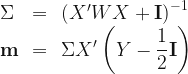
Therefore, by introducing Polyá-Gamma random variables, the Gibbs sampler proceeds by repeating sampling from the following two distributions
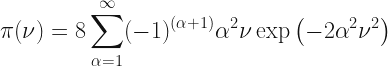
Next method is using the hierarchical representation of the logistic distribution as a scale mixture of normal as proposed in Stefanski (1991). That is the logistic PDF can be recast as
![f(x) = \dfrac{e^{-x}}{(1+e^{-x})^{2}} = \displaystyle \int_{0}^{\infty} \left[\dfrac{1}{2\nu\sqrt{2\pi}}\exp\left\{-\dfrac{1}{2}\left(\dfrac{x}{2\nu} \right)^{2} \right\} \right]\pi(\nu)\,d\nu](https://s0.wp.com/latex.php?latex=f%28x%29+%3D+%5Cdfrac%7Be%5E%7B-x%7D%7D%7B%281%2Be%5E%7B-x%7D%29%5E%7B2%7D%7D+%3D+%5Cdisplaystyle+%5Cint_%7B0%7D%5E%7B%5Cinfty%7D+%5Cleft%5B%5Cdfrac%7B1%7D%7B2%5Cnu%5Csqrt%7B2%5Cpi%7D%7D%5Cexp%5Cleft%5C%7B-%5Cdfrac%7B1%7D%7B2%7D%5Cleft%28%5Cdfrac%7Bx%7D%7B2%5Cnu%7D+%5Cright%29%5E%7B2%7D+%5Cright%5C%7D+%5Cright%5D%5Cpi%28%5Cnu%29%5C%2Cd%5Cnu+&bg=%23ffffff&fg=%23111111&s=2&c=20201002)
where 
This time we don’t model the regression model directly but we will rather resort to the latent variable representation. That is, we will assume there is a latent variable 


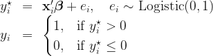
We merely replace 

![\pi(\boldsymbol{\beta},\nu\,|\,Y) = \left[\displaystyle\prod_{i=1}^{n}\left(\mathbb{I}\left(y_{i}^{\star}>0\right)\mathbb{I}\left(y_{i}=1\right)+\mathbb{I}\left(y_{i}^{\star}\leq 0\right)\mathbb{I}\left(y_{i}=0\right)\right)\dfrac{1}{2\nu}\phi\left(\dfrac{y_{i}^{\star}-\mathbf{x}'\boldsymbol{\beta}}{2\nu}\right)\right]\pi(\boldsymbol{\beta},\nu)](https://s0.wp.com/latex.php?latex=%C2%A0%5Cpi%28%5Cboldsymbol%7B%5Cbeta%7D%2C%5Cnu%5C%2C%7C%5C%2CY%29+%3D+%5Cleft%5B%5Cdisplaystyle%5Cprod_%7Bi%3D1%7D%5E%7Bn%7D%5Cleft%28%5Cmathbb%7BI%7D%5Cleft%28y_%7Bi%7D%5E%7B%5Cstar%7D%3E0%5Cright%29%5Cmathbb%7BI%7D%5Cleft%28y_%7Bi%7D%3D1%5Cright%29%2B%5Cmathbb%7BI%7D%5Cleft%28y_%7Bi%7D%5E%7B%5Cstar%7D%5Cleq+0%5Cright%29%5Cmathbb%7BI%7D%5Cleft%28y_%7Bi%7D%3D0%5Cright%29%5Cright%29%5Cdfrac%7B1%7D%7B2%5Cnu%7D%5Cphi%5Cleft%28%5Cdfrac%7By_%7Bi%7D%5E%7B%5Cstar%7D-%5Cmathbf%7Bx%7D%27%5Cboldsymbol%7B%5Cbeta%7D%7D%7B2%5Cnu%7D%5Cright%29%5Cright%5D%5Cpi%28%5Cboldsymbol%7B%5Cbeta%7D%2C%5Cnu%29++&bg=%23ffffff&fg=%23111111&s=1&c=20201002)
The key point to remember is that if we change our perspective about the order in which 


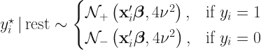
where 

Next is 

So I have reviewed 2 modelling methods for Bayesian logistic regression and they both have advantages. However, I would say the Kolmogorov-Smirnov modelling is more general in the sense that it can be used with more complex models such as nonparametric regression.
For the samplers, I have Matlab codes here.
- Choi, H. M., & Hobert, J. P. (2013). The Polya-Gamma Gibbs sampler for Bayesian logistic regression is uniformly ergodic. Electronic Journal of Statistics, 7, 2054-2064.
- “Non-Uniform Random Variate Generation, Luc Devroye, Springer-Verlag, 1986,
the University of California, 16 Dec 2010, ISBN:0387963057, 9780387963051” - Stefanski, L. A. (1991). A normal scale mixture representation of the logistic distribution. Statistics & Probability Letters, 11(1), 69-70.

very helpful thx
LikeLiked by 1 person